Before you start pruning and cleaning your data, you need to have a clear idea of what you want to be doing with it. Ask yourself what features are going to be relevant to your analysis and what you can write off. For our case study, we will be trying to find out how many food products in our dataset contain palm oil or ingredients that may be from palm oil. This means that most of the columns already in the data won’t be useful. Since we are working on Google Sheets, we will first start by duplicating the tab so we have a copy of the original data. Then we will remove all columns that we know we won’t be needing later on (which happens to be most of them in this scenario). We will be getting rid of information like product codes, contributor, and other extraneous nutritional information. We will, however, keep information about the countries, brands, and important nutritional values like protein, carb and fat content, since these could be interesting features to study. Always err on the safe side and keep anything that you suspect might be useful later on. This leaves us with 41 columns from the 106 we had originally.
Often, when one is working with datasets such as this one, some records will be missing information due to the fact that contributors did not provide the information. This might mean only certain features are missing on some records, or that some records have so little information as to be unusable.
We have two options when dealing with null values in the data:
Let’s take a look at our example: the OpenFoodFacts Dataset is full of holes regarding the nutritional content of the foods recorded. When deciding what to do with those records, it is very important to have in mind what you’re trying to achieve with the data. If you’re studying people’s heights across the country, then you can get rid of any entries where the height hasn’t been recorded.
In our case, since we’re trying to study the palm oil content of products, any records that don’t have any data relevant to palm oil content are useless to us. First, we see that there are a few columns relevant to this:
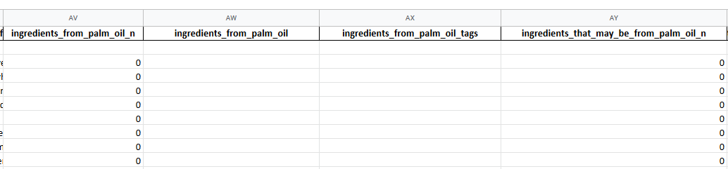
In these columns, we can see that the ones supposed to contain the names of ingredients are empty or almost empty, so we can already decide to get rid of them. What is more interesting is looking at the number of ingredients containing palm oil or that may contain palm oil. Therefore, we will be getting rid of any records where neither column has any information. Now, this doesn’t mean you should go and manually check all 2000 records one by one. Since we’re using Google Sheets for this exercise, we will rely on the very powerful FILTER function to do the job for us.
To filter out unusable rows, we will do the following:
What this formula does is filter the A to AO range of columns from our pruned dataset, and only keep rows if the X column (number of ingredients from palm oil) or (here represented by the logical + operator) the Y column are numbers (which is determined by the handy ISNUMBER function). This ensures that only records where a number of ingredients have been specified are kept, and that everything else is omitted. We could also have used other logical conditions to filter out blank values if we hadn’t been dealing with a numerical feature.
As you may have noticed, we haven’t removed the columns containing the timestamps for the creation of the records, even though they would not be very useful for the kind of analysis we’re working on. We will use them as an example to show how we can deal with time data and convert it into a compatible format. Both columns show timestamps in formats that aren’t natively supported by Google Sheets, namely Unix Epoch Timestamps and ISO format.

Since it is easier to deal with the Unix timestamps on Google sheets, that’s what we will be converting. In this case, we’ll add a column to the sheet, and use the following formula to convert the timestamp into the Datetime format used by Google Sheets:
=arrayformula(B2:B/86400+date(1970,1,1))
The ARRAYFORMULA function allows us to spread the function to the whole column. If you don’t know what type of time format is used in a dataset, there are tools online that allow you to convert and find out what standard is being used.
With categorical data, particularly in datasets where the data has been collected from users directly, we might notice that different denominations are used to refer to the same category. For instance, this dataset contains information about the country of origin of the products, and if we take a look at the “countries” column, we can see that the same country can be referred to in multiple different ways. In order to correct this, we will look at all the unique values this column takes by using the UNIQUE function on the column.
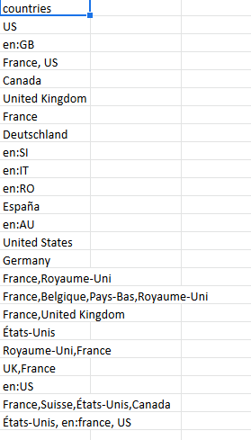
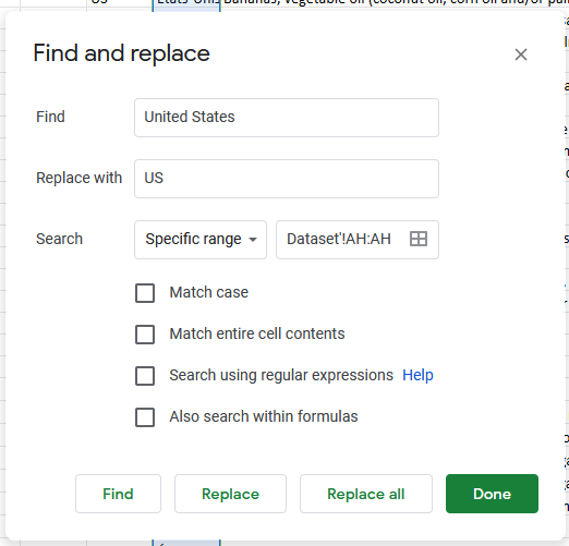
What we see here is that countries have been recorded in multiple ways. In order to standardize these categories, we can use the find and replace feature and decide on a single way to refer to each of the countries present in the list.
Outliers in the data are tricky to define, and the way they are handled will greatly depend on what you are trying to do with your data and what it represents. When building a forecasting model for a website’s traffic, for example, it can be useful to remove spikes that may skew the model if we are sure they are one time events. If studying heights, a record showing someone who is 18 meters tall instead of 1.8m tall is a simply typo and needs to either be removed or corrected. Since we can’t check each record individually, a good practice is to check the maximum, minimum, and mean values of numerical features, and deal with any outliers accordingly.
Let’s take for example the “ingredients that might be from palm oil column”. We will check the max, min and mean of this column (using the MAX, MIN and AVERAGE functions):
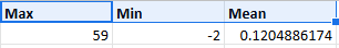
Here we see that these values don’t seem correct, since it is unlikely any product has 59 ingredients from palm oil, and it is impossible for that value to be -2 since the number can’t be negative.
We use a filter again, with the following formula:
=FILTER('Step 2-3: Remove Blanks, Convert Times'!A2:AO, 'Step 2-3: Remove Blanks, Convert Times'!Y2:Y>=0,'Step 2-3: Remove Blanks, Convert Times'!Y2:Y<10)
Here we’re telling the filter to only keep rows where the number of ingredients is positive and less than 10.
Once all these steps are done, we have a dataset with 41 columns and 1796 rows, that at a glance looks much more dense and not as sparse as the original. We have managed to only retain features that would be useful to our purpose, remove records with insufficient data, get rid of outliers and errors and standardize the categories. With this, working on the data and extracting insightful information from it will be much easier, and the chance of making mistakes due to incongruities in the data are minimized. These same steps apply to almost any kind of dataset, and as long as one has a good grasp of the data at hand and what they plan on doing with it, the rest is merely a matter of finding the right tools to shape the raw data into a diamond of insights.